BLOG 3: DESIGN OF EXPERIMENT

Updated: Jan 26, 2025
WELCOME BACK TO MY BLOG.
New year, old me. I hope all my readers have had an enjoyable and restful break over the December holidays, I sure made the most of it. Or that's how it felt to me at least. But all good things must come to an end. And so we find ourselves back in the lab again, walking down that same familiar yet unfamiliar path into discovery and study. As melancholy as that opener sounds, this term looks pretty jam-packed with learning all sorts of new and interesting things. Maybe a bit too much jam for my taste but it is what it is. Even a big opportunity to put our learning into practice on our terms! But I won't spill all the beans here, just know that there's lots of excitement working its way down the blog pipeline.
DESIGN OF EXPERIMENT: FOR DUMMIES
Contrary to its name Design of Experiment (DoE for short) isn't actually about designing the experimental procedure itself, well it kind of is. But not really? Just let me explain it will make a lot more sense in a minute.

In technical jargon, DoE is described as a "Methodology to obtain knowledge of a complex, the the
multi-variable process with the fewest trials possible."
I'm sure that sentence is comparable to ancient hieroglyphics to you guys, it sure was for me during my first time reading it, so let me put it in terms of a very very relatable metaphor. Imagine you are an overworked, sleep-deprived, cortisol-filled, dateline-chasing Chemical Engineering student, "Actually I, unfortunately, do not have to imagine, but you get the point" As such your survival hinges on the liquid gold that is Teh or Kopi, pick your poison. The

only thing that's keeping you awake as you fight off the adenosine and cortisol build-up to meet datelines you evidently should have started on ages ago. That steaming cup in your hand is more than just a source of caffeine, it's truly only the last tiny slither of joy left in your day-to-day endeavors. The Chemical Engineer in you decides to try and optimise the brewing process so that you can get the most delicious and enjoyable mug of joy in the shortest time possible. "remember you're chasing datelines so you don't have time to waste" Alas, with your enlightened engineering perspective, you know that even something as simple as brewing coffee or teh is complex with many variables that have to be manipulated intricately to distill the brown elixir of life that is perfectly suited to your tastes. Brew time, brew temperature, type of bean or leaf, and the size of said bean or leaf. All play major roles in things like flavour, texture, bitterness, and aroma all of which you have a specific preference for. "SO MANY VARIABLES SO LITTLE TIME! HOW?" Very appropriate response for someone who does not have time on their side. So how can we overcome this, we simply cannot afford to run god knows how many experiments with different levels on each variable just hoping to strike 4D and find the ideal one by chance. A foolish decision both in the monetary and time sense. So this is where DoE comes in. Instead of running dozens of experiments on all the factors we can simply run all the factors in the same experiment at various levels so that we can observe the effect of each factor on our desired outcome, in this case how each factor affects the flavor, texture, bitterness, and aroma. "Even with this methodology or whatever sorcery I'd still have to run 16 different experiments and that's without any repeats for consistency. So how exactly does this help me?"

Well, why don't you just do half of them and leave the other half for later? As much as that sounds like a joke, the magical part is that it isn't. This is where statistics comes in, yeah sure you could do all 16 different experiments at the bare minimum for 3 repeats for a total of 48 runs and have 100% confidence in your results. (this is called a full factorial design btw)
But would it be so bad to only have to do 24 runs but only have 90% confidence in your results? My wallet and sanity sure know which one they prefer.
But which experiments should we choose? And how do we know we still have that 90% confidence? To know that we have to talk about geometry, a lot of tangents in this blog. I know For our results to retain good statistical properties we must choose a orthogonal design of experiments. That means that all the factors/variables that we are investigating occur the same number of times at both their high and low levels.
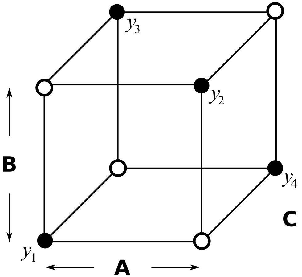
The images here show an example of an orthogonally balanced design of the experiment. As you can see from the table below. The number of times each factor is high is equal to the number of times that each factor is low. This will ensure a balanced experiment and thus good statistical properties in the data that we collect. (this is called a fractional factorial design)

Since our data has good statistical properties we can say with a reasonable amount of confidence that the trends we observe in this smaller set of data will be similar or ideally the same as the trends we will see in the larger set of data. Hence, allowing us to reach the same conclusion about the effect of a certain factor, but with much less time, energy, and, most importantly, money spent!
TALK IS CHEAP, JUST LIKE MY 70-CENT TEH AT FC1
So let us put whatever we may have gleaned from the above section into practice.
So let us examine a case study for which data has already been provided for us.

In this case study 8 runs were performed where 100 grams of corn was used in each experimental run and the measured variable was the mass of "bullets" formed, The bullets in this case refer to the tiny little bits of unpopped kernels of corn. As such it is clear that the main goal of this experiment is to determine the ideal conditions under which the smallest mass of bullets is obtained. Or the greatest amount of popcorn is popped. Three different factors were varied in this study. Factor A, the diameter of the bowl used to contain the unpopped kernels (10 and 15cm) Factor B, Microwaving time (4 minutes and 6 minutes) Factor C, The power setting of the microwave (75% and 100%) All 3 factors were varied at two distinct levels and shall henceforth be referred to as Low (-) or High(+) levels.
FULL FACTORIAL STUDY
To ascertain the effectiveness of utilising DoE we must do both a full factorial (using all the data) and a half factorial (using half the data, ensuring this data is orthogonally balanced) and then make a comparison of the trends obtained by the two different methods.

To determine the effect of changing a certain factor. We must first find the mean of the measured variable in all experimental runs at both of its distinct levels. For example, we must find the mean of all the runs where Factor A is high (The diameter of the bowl is 15cm) and the mean of all the runs where Factor A is low (The diameter of the bowl is 10cm). Having plotted this data we can already start to draw some conclusions based on it. As the diameter of the bowl increased from 10cm to 15cm, the average mass of bullets decreased from 1.89g to 1.7425g indicating an increase in the amount of kernels that were popped. As the microwaving time increased from 4 minutes to 6 minutes, the average mass of bullets decreased from 2.165g to 1.4675g yet again indicating an increase in the amount of kernels that were popped. As the microwave's power increased from 75% to 100%, the average mass of the bullets decreased from 2.9175g to only 0.715g also indicating an increase in the amount of kernels that were popped. Having done this in the table above for all conditions we can then plot these factors linearly on a graph against the average mass of bullets formed in grams to visualise the effects more clearly.

From the above graph which we have plotted, we can start to draw some conclusions about the effect of each factor on the average mass of bullets. Using the gradient of each line, a steeper gradient will indicate a larger change in the average mass of bullets and thus can be used to quantify the effect of the factor itself on the measured variable.
The most influential factor affecting the mass of bullets is the microwave's power (factor C). This can be seen in the graph in the form of the gradient of its linear line being the steepest at -2.2025 indicating a very significant change as its level changes from high to low,
followed by the Microwaving time (factor B) with a gradient of -0.6975.
The diameter of the bowl is in last place (factor A) with a gentle gradient of -0.1475.
"But how do you know if two factors are working together to produce a better result or against one another to diminish your results" Very astute observation and a really good question. To do so we must compare the data with itself again. This time to compare the effect of two factors we must plot one factor at two levels against another factor at both of its levels to determine if they are interacting.
Let us do this for factors A and B, by first collating the data points for which factor A is high and low while factor B is high concurrently. We repeat this collection for which factor B is low throughout and factor A is both high and low. "This is a mouthful, huh, I hope the data table below makes it make more sense"

From the data above we can begin to observe pretty interesting things already. When B is high, the change in factor A from High to Low results in a decrease in the average mass of bullets as evident from the negative difference of 0.765g. However, when B is low changing factor A from high to low results in a positive difference of 0.47g indicating an increase in the average mass of bullets formed. To further make things clearer for our observations we can plot these on a graph to better visualise it.

As we can see from the graph, the gradients of both lines are significantly different, one is positive while the other is negative. This indicates that there is a significant interaction between Factors A and B. We can then proceed to repeat this for the other two sets of factor interactions.
For factors A and C. The data collated is displayed in the table below.

Observing the data we can see that, Changing factor A from a high to low level at a high C results in a difference of -0.16g meaning a decrease in the average mass of bullets formed. Changing factor A from a high to low level at a low C results in a difference of -0.135g meaning a decrease in the average mass of bullets formed as well. Visualising the data.

We can see from the graph that the gradients of both lines are only very slightly different, also evident from the very close gradient values, indicating that there is an interaction between A and C but it is soooo small that it is essentially negligible.
For factors B and C. The data collated is displayed in the table below.

Making observations, We can see that when changing factor C from High to Low at a High B, the difference in the average mass of bullets is -1.765 indicating a decrease.
We can see that when changing factor C from High to Low at a Low B, the difference in the average mass of bullets is -2.64 indicating an even greater decrease.
Visualising the data.

From the graph above we can see that, the gradients of both lines are quite different indicating that there is a measurable interaction between factors B and C, as evident from the different slope values of -1.135 for factor C low and -0.26 for factor C high.
After examining all the numbers we can summarise them into a few key findings. For all factors, increasing them from a low to a high-level results in the average mass of bullets decreasing. meaning increasing any one of them or all of them or just a few of them will generally result in a lower average mass of bullets thus meaning more edible popcorn. Increasing the microwave's power will result in the greatest decrease in the amount of unedible popcorn followed by time in the microwave and with the diameter of the bowl resulting in the smallest change.
However, before we can truly decide the most ideal conditions for popping of pop-corn we must keep in mind the interactions. As we have discovered, The most significant interactions exist between factors A and B. While there are still interactions between factors A and C and factors B and C Observing the graphs for the interactions between factors A and C and the interactions between factors B and C, their interactions are not as significant as the interaction between factors A and B which is evident from their graphs which do not show any super significant changes in gradient. However, Analysing the data between factors A and B it is notable that increasing the plate diameter is much more effective when we also increase the microwave time as the gradient for the line where A is high. Still, B is switched between high and low is the steepest showing the greatest change. After considering all of these factors we can conclude that the most significant reductions in the mass of bullets will come from either increasing the microwave power or increasing both the plate diameter and time spent in the microwave. With the most effective conditions are the combination of all 3 factors being at a high level.
HALF FACTORIAL ANALYSIS
We've finished our analysis of the full data, now let's see if we can do half the work but still see the full picture.
Before we dive into analysing and plotting graphs we must choose our data wisely. As you'll recall for half factorial analysis to be statistically viable we must choose data that is orthogonally balanced.
(Basically, high and low factors must be investigated the same number of times if you weren't paying attention earlier)
When deciding the half-factorial of runs you could either choose runs 1,2,3 and 6. as shown below.

Or you could just as easily choose the opposite runs of 4,5,7 and 8 and still have an orthogonally balanced layout.

But for our analysis, I will be sticking with runs 4,5,7 and 8. "Thankfully, the tables I have poured my heart and soul into making can be reused if we simply remove the runs that are not being used"

Examining the table we can make some preliminary observations again. As the diameter of the bowl increased from 10cm to 15cm, the average mass of bullets decreased from 0.9925g to 0.7g indicating an increase in the amount of kernels that were popped. As the microwaving time increased from 4 minutes to 6 minutes, the average mass of bullets decreased from 1.0175g to 0.675g yet again indicating an increase in the amount of kernels that were popped. As the microwave's power increased from 75% to 100%, the average mass of the bullets decreased from 1.2425g to only 0.45g also indicating an increase in the amount of kernels that were popped. Comparing this to the full factorial design we can already glean a similar trend of all factors increasing resulting in a general decrease in the average mass of bullets formed.
But a picture carries the weight of a thousand words. Well, a graph should carry the weight of like a million words then.

Examining the graph we can see that the most influential factor is the Microwave's power (factor C) as quantified by the gradient of its line as it has the steepest gradient with a value of -0.7925.
Followed by microwaving time (factor B) with a gradient value of -0.3425
In last place, we have the diameter of the bowl (factor A) with a gentle gradient value of -0.2925
COMPARING FULL FACTORIAL AND HALF FACTORIAL
This is once again similar to what we have observed in the full factorial investigation. The influence ranking of all the factors has continued to follow a similar trend. However, upon closer inspection of the data values themselves, we can see while the data seems to follow a trend the magnitude of these effects is quite different in the full factorial.
Gradient/Effect | Factor A | Factor B | Factor C |
Full Factorial | -0.1475 | -0.6975 | -2.2025 |
Half Factorial | -0.2925 | -0.3425 | -0.7925 |
Looking at this table it's easy to see the fact that the magnitude of the effect of each factor is much different in the full factorial study than in the half factorial study. This highlights the weakness of using a half-factorial study. The reduced number of data points leaves the experiment more sensitive to random variability that may simply be the result of factors outside of the experimenter's control. Thus creating a bias in the set of data. Despite this, the results stayed relatively consistent in displaying a similar trend and this shows us that often these trends are more than enough to come up with meaningful conclusions that aid the experimenter in answering the question they have asked to begin with.
Conclusion and learning points
To conclude this extremely theory-heavy blog, I'd like to spend some time reflecting and sharing with you my learning points.
The first learning point I've gleaned from this is that it's important to know how to present and show your data. Many times I've reformatted and rewritten parts of this blog and completely revamped my Excel sheet because whenever I would look at it I would just think that "this would not make any sense to anyone but me". And it threw me back to when I'm doing research for my other modules I often come across sources with data that is either so poorly formatted or just utterly incomprehensible that you just don't know what to make of it.
So after being on the other end and being the one trying to showcase your data to other people outside yourself. I've grown a new sense of appreciation for keeping things tidy and simple so that even if someone who has no idea what you're talking about were to open your spreadsheet and have a glance they could have at the very least a rough idea of what is going on and how the numbers are useful to them.
Another learning point I've ascertained is that engineers are lazy. Well, not exactly, it's just that they are the epitome of the phrase "work smart, not hard". When faced with something that is so obscenely taxing mentally like doing hundreds of runs of experiments these clever little buggers have come up with a method of even doing that more lazily. But results are results and honestly, I don't think anyone can complain if you can attain the same result but with less effort. Especially if money is involved.
A more technical final learning point I want to share with you guys is that there is always a trade-off. Always always always, even just looking at the case study I've covered in this blog it is blatantly apparent that you simply cannot have it all. If you're going to save yourself time and do the fractional result to meet a dateline or simply because you lack the human or monetary resources that's fine. But be completely prepared to give up the accuracy of your data as well as any knowledge on the interaction between factors of your given experiment.
In my opinion, choosing between a fractional and full factorial DoE comes down to the nature of the experiment itself, in the context of what we've done for our practical where our experiment was as simple as shooting toy catapults repeatedly with just a few changes here and there it makes sense to just do the full factorial and have a completely accurate set of data. But let's say the experiment isn't just as easy to repeat or god forbid, expensive to carry out. Then it just makes sense to rely on a fractional factorial.
Another factor to consider when choosing between a fractional and full factorial DoE is whether the data on the interactions between factors is important. Sometimes, knowing the interactions between factors can be the difference between saving a pretty penny on certain large-scale processes so in that sort of context it makes sense to just invest a large amount of capital and effort in performing the full factorial to get data you're confident in and the correlations between them. So that more money can be saved by the adjustments made post-experiment in the long-term.
I suppose it all comes down to the situation that you're in and the decisional trade-offs you're willing to make but there always will be a trade-off. You simply cannot have it all.
AND WITH THAT WE'VE COME TO THE END OF BLOG 3. I want to acknowledge that maybe this blog hasn't exactly been the most engaging or the most witty one I've written to date. I'm not going to make any excuses I've just not been feeling it lately. But I still hope that you've stuck around till the end and at the very very least learned a little bit of something new or maybe laughed at one of the few witty comments in this blog. Either way, I hope you're doing well and continue to do so. There's still one more blog left so still stay tuned until next time. Peace Also i've embedded the excel file i've used below so have a look if you'd like


Comments